Rhonda Hamilton Case Scenario
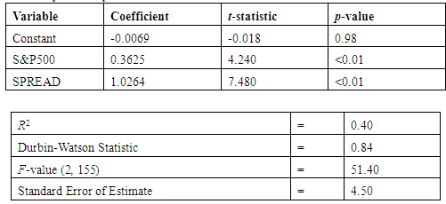
Rhonda Hamilton, CFA, manages the Select Electric Fund. Hamilton is reviewing a research report written by Brian Ender about the U.S. electric utility industry. Ender’s report includes the regression model and relevant statistics presented in Exhibit 1. The dependent variable for the model is the monthly return for an electric utility equity index for the previous 158 months. The independent variables are the monthly returns for the Standard & Poor’s 500 (S&P500) and the difference between the monthly returns on long-term U.S. government bonds and one-month U.S. Treasury bills (SPREAD). All variables are recorded in percent.
Exhibit 1
Ender’s Regression Model
Electric Utility Industry

Ender’s report concludes that the model is well-specified because its explanatory power is good. The report also contains a footnote indicating that confidence intervals for predicted utility equity returns can be easily computed using only the standard error of estimate.
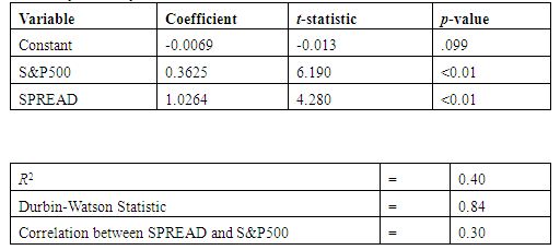
Hamilton agrees that S&P500 and SPREAD are reasonable independent variables, but she is not convinced by Ender’s conclusions. Using Ender’s data, Hamilton tested for and confirmed the presence of conditional heteroskedasticity. She then ran a regression similar to that run by Ender and corrected for conditional heteroskedasticity using robust standard errors (i.e., Hansen’s method). Hamilton’s regression model and relevant statistics are presented in Exhibit 2.
Exhibit 2
Hamilton’s Regression Model
Electric Utility Industry

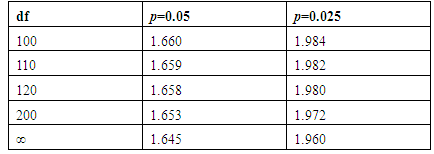
Hamilton hypothesizes that the returns for the electric utility equity index have a sensitivity coefficient to bond yields (i.e., SPREAD) equal to one. She is also interested in the precision of the sensitivity of electric utility equity returns to S&P500. Hamilton wants to use the regression results to address both of these issues. Selected values of the t-distribution are shown in Exhibit 3.
Exhibit 3
Selected Values of the t-Distribution
(Degrees of freedom = df, one-tailed probabilities = p)

1) Given Hamilton’s finding regarding heteroskedasticity, the most appropriate conclusion is that the variance of the error term is:
A. correlated with the values of the dependent variable.
B. correlated with the values of the independent variables.
C. not correlated with the values of the dependent variable.
D. not correlated with the values of the independent variables.
2)If Hamilton assumes that the monthly values for both SPREAD and S&P500 are 1%, the predicted monthly return for the electric utility equity index is closest to:
A. 0.36%.
B. 1.00%.
C. 1.03%.
D. 1.38%.
3)In assessing how well her regression model explains electric utility equity index returns,
Hamilton’s most appropriate conclusion is that:
A. 16% of the variation in index returns is explained by the regression model.
B. 36% of the variation in index returns is explained by the regression model.
C. 40% of the variation in index returns is not explained by the regression model.
D. 60% of the variation in index returns is not explained by the regression model.
4)Based on the results in Exhibit 2, the value of the test statistic relating to Hamilton’s null hypothesis about the value of the sensitivity coefficient to SPREAD is closest to:
A. 0.11.
B. 0.24.
C. 4.17.
D. 4.28.
5)Based on the results in Exhibit 2, if degrees of freedom = 200, the 95% confidence interval for the sensitivity of electric utility equity index returns to S&P500 is closest to:
A. 0.19 to 0.53.
B. 0.22 to 0.50.
C. 0.25 to 0.48.
D. 0.27 to 0.46.


